
Papers: Dynamic Programming with Zombies and Pirates
Dynamic Programming was developed by Richard Bellman while he was working for The RAND Corporation in the 1950’s. During this time The RAND Corporation was employed by the Air Force. In his autobiography Bellman describes his reasoning for the name dynamic programming; the Secretary of Defense at the time, Wilson, “had a pathological fear and hatred of the word, research” [sic]. As a result the name was picked to shield what Bellman was doing within The RAND Corporation. In 1979 Bellman was awarded the IEEE Medal of Honor for the creation of dynamic programming.
Dynamic Programming is the process to solve a problem based on overlapping sub-problems, and it can be either top-down or bottom-up. Top-down approach to dynamic programming breaks down the main problem into sub-problems and will solve the sub-problems to get the solution to the main problem. A top-down solution makes use of recursion and memoization. Memoization is remembering of solutions to certain sub-problems, often in an array, so they do not need to be solved again. Comparatively a bottom-up solution is when all sub-problems are solved in advance and later used to form solutions to larger problems made up of those sub-problems. Top-down starts with the main problem and will work “down” towards the sub-problems whereas the bottom-up approach starts at the sub-problems and works to the “top” main problem.
An example of a problem that can be solved by using dynamic programming is the Roaming Zombie problem. A zombie is in a city and is hungry so he wishes to find a brain. Zombies are slow and in order to get to the brain as fast as possible the zombie must follow the shortest path he can to reach the brain.
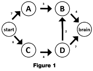
Figure 1 shows a directed acyclic graph (DAG) of the possible ways the zombie can reach the brain. Using a bottom-up approach in solving this problem we start at the brain and work backwards to the starting point. From each point we find the shortest path to the brain from it. For example from the point brain to brain the shortest distance is zero with the path of nothing because we are already at the desired ending point. From B to the brain we only have one option of going to the brain which gives us a distance of four. Continuing backwards we are at D and we wish to go to the brain. We can either go from D to B or from D straight to the brain. From D to B we travel a distance of two plus the total distance from B to the brain which we already determined was four giving a total of six. From D to the brain we travel a distance of seven. As six is shorter than seven we note that the shortest distance from D to the brain is six and that the path to take is D → B → Brain. Building upon the previous sub-problems we can build a solution to the entire problem.
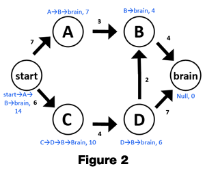
Figure 2 shows the solutions to the sub-problems. Continuing to work backwards from where we left off node A has only one option for which path to take so we take the solution from B and add it to A → B to get seven for the optimal distance and a path of A → B → brain. From C we also only have one option. So we take the optimal path from D and add the distance of from C → D to it. The distance in this case is ten. The path is C → D → B → brain. Looking at this you can see that the shortest path from the starting position to the brain is from start → A → B → brain and that the distance traveled is fourteen. Each node contains above or below it the optimal path and distance that the path would cover. Where there is more than one option for the path to follow, as in the case of the starting position, we look the two options and see what the optimal path in each case is and pick the minimum of the two.
Another problem that can be solved using dynamic programming is The Pirate Chest problem, a variation on the common Knapsack Problem. This problem can be solved by using a top-down approach to dynamic programming. The pirate Captain Kidd is the only pirate known to have buried his treasure. Captain Kidd has N types of treasure of varying cost and size and a treasure chest that can hold a capacity of M. All items not put in the treasure chest will be spent immediately or split up amongst the other pirates. We need to find a combination of items so that Captain Kidd can maximize his savings.
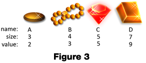
Figure 3 shows the items that Captain Kidd has to choose from for his treasure chest as well as the size and value of each item. The items have been given names A, B, C, and D for simplicity.
Rather than selecting items just to maximize the usage of the area in the treasure chest we need to select items that utilize the most area while getting the most value for that area.
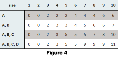
Figure 4 shows the solution for the problem. Note that the sub-problems in this case are the items that are available to choose from. Starting with using only A’s then A’s and B’s then A’s, B’s and C’s and finally all four possible items. The values written in the table is the maximum value that can be stored in the treasure chest.
The algorithm to find the solution is to first note the largest sized item in the current grouping. In the first row of Figure four there is only one item so the size to keep in mind here is three. If the size is less than the size of the item no items can be stored so our first two columns in the first row are zero. Once we hit a number over our item size we can finally start storing items. We cannot store partial items so from size three through size five we can hold one A giving a value of two. Once we hit a size of six we can start storing two A’s for a value of four. Our program has no way to evaluate the problem in the same way that the human mind would, so another way of knowing this is to examine the size that it can carry, in this case 6, and subtract the size of the largest item (three) to get a value of three. We look in our matrix under three to find that the left over space can hold a value of two. The addition of the value of the largest item plus the value the left over space can hold will give us the total value the current size is able to hold. If we simplify this statement into an equation we have: Value(Size) = Value(Size – ItemSize) + ItemValue, where Value(Size) will give the value using all available items at a given size and ItemSize is the size of the largest item we are able to use. We also need to check the value of the column in the row above the current row. The algorithm is as follows:
int treasure(int[] size, int[] value, int n, int m){
  	if(n==0)
    		return 0;

 	if(m - size[n] < 0)
    		return treasure(size, value, n-1, m);
  	else
    		return max(treasure(size, value, n-1, m), treasure(size, value, n-1, m - size[n]));
}
The function treasure takes four values: size, value, n, and m. Size and value are both arrays containing the sizes and values for each of the items. The integer n is the item number in our case we would map A, B, C, and D to 1, 2, 3, and 4. The integer m is the size of the treasure chest. If we modify the above code to remember the values of previously solved sub-problems using memoization we can prevent the program from doing work repeatedly. This can be done by creating an array of the sub-problems and their values and adding a check in the beginning to see if the solution to the sub-problem exists in the array.
A problem that can readily be solved by using dynamic programming and the application of memoization is the Fibonacci sequence. The problem becomes a little more interesting when you add in the concept of population growth. In our first example we saw a zombie coming for a human brain now we are going to look at how these zombies multiply. We have learned in “Dawn of the Dead” and other Hollywood movies the zombies multiply by biting humans.
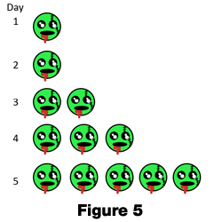
Figure 5 shows the population growth of zombies over time. As you need to start with one zombie in order to make more, the population at day one is one. At day two our population is still one because he got lost in a DAG and was unable to find any brains to eat. On day three our first zombie finally goes and makes another one to give us two zombies. Day four our new zombie creates another one so we have three. On day five our two new zombies create new ones to give us a total of five. We can simplify the model of the population growth of the zombies by the statement the total of zombies on any day is the sum of total of zombies the two days before it. However, on days one and two our first zombie is alone so it is important to note that the total will be one on those days. Mathematically put: Total(Day) = Total(Day-1) + Total(Day-2) if Day > 2, otherwise Total(Day)= 1. When shown as a statement to this a recursive method is easy to see and we get the following code:
int total(int n){
  	if(n == 1 || n == 2)
    		return 1;
  	else
    		return total(n-1) + total(n-2);
}
The above code has issues with it, sure it was the easiest to see of the solutions to the problem of finding zombie population on a given day, but a lot of work is done multiple times. To find the size of the zombie population at day five we need to find the size of the population at days four and three. To find the population on day four we need to find the population on day three and day two. Then later on in finding the solution we need to find the population for day three again. By adding memoization to the above problem we can save time and thus have more time to prepare for the coming zombie apocalypse as at this rate the population will grow very fast. The following code has the addition of memoization to prevent repeated work.
static int[] memo = new int[MAX];
int total(int n){
  	if(memo[n] != 0)
    		return memo[n];

  	int pop;

  	if(n == 1 || n == 2)
    		pop = 1;
  	else
    		pop = total(n-1) + total(n-2);

  	memo[n] = pop;
  	return pop;
}
We start out with an array outside of the function that will store sub-problems that we have already solved. When we first enter the function we check if we have done the work already, if we have then we return it. In cases where we have not done the work already, we do it and then we store it in our array and return the discovered value. This eliminates all repeated work.
As we have seen in the above examples dynamic programming takes larger problems and breaks them up into easy to solve pieces to build up a whole. The two approaches to dynamic programming allow us to work with a problem in a bottom-up fashion or a top-down fashion. In the three examples we have seen how different problems can be solved by using the idea of dynamic programming. We have also seen that recursive solutions to these problems often benefit from the usage of memoization. Since its creation nearly 50 years ago dynamic programming has affected how we approach solutions to problems.
References
- Bellman, Richard. Eye of the Hurricane. Singapore: World Scientific Publishing Company: 1984.
- “Richard Bellman, 1920 – 1984.” IEEE.<http://www.ieee.org/web/aboutus/history_center/biography/bellman.html>. archive
- Sedgewick, Robert. Algorithms in C++. Massachusetts: Addison-Wesley Publishing Company,1992.